A visualization of latent space distance models for Graphs
February 1, 2022
In this article I give a visualization of latent space distance models for graphs, and how they allow to disantangle the metric structure of the graph from prior information such as node/edge attributes.
Introduction
Latent space distance models for graphs form a broad class of statistical models for graph. In what follows we give a visual explanation of the mechanisms that allow these models to disantangle different effects in the network generation process.
Latent space models for graphs (LSM)
$\newcommand{\Zcal}{\mathcal{Z}}$ Given a graph $G=(U,E)$ where $U$ is a set of nodes and $E\subset U\times U$ is the set of edges of $G$, a LSM supposes for each node $i\in U$ the existence of an underlying latent representation $z_{i}$ in a metric space $\Zcal$. We denote by $y_{ij}$ the (binary) indicator that the edge $ij$ is in $E$.
Then, supposed that the edges $ij$ in the network are independently generated by a Bernoulli distributions $Bern(\theta_{ij})$, such that: $$\theta_{ij} = f(z_i, z_j)$$ for a certain similarity function $f$.
Examples of Latent Space models include the stochastic block model, where the embeddings are discrete, the graphon model (Lovász, 2012), and the Latent space distance model introduced in (Hoff et al., 2002).
Latent space distance models (LSDM)
Here we focus on the generic latent space distance models, presented in (Hoff et al., 2002). Those are such that the similarity function is composed by a logit passed through an activation function $h$ (Usually the sigmoid function):
$$a_{ij} \sim Bernoulli(\theta_{ij}) $$ $$\theta_{ij} = h(2\gamma +\alpha_i + \alpha_j+ \lambda^Tx_{ij} - d(z_i,z_j))$$
Where $\alpha_i$ and $\alpha_j$ sociality parameters, $x_{ij}$ are predefined edge features, $\gamma$ is a bias parameter and $d$ is a distance, such as the euclidean distance.
Deterministic version of the random graphs above.
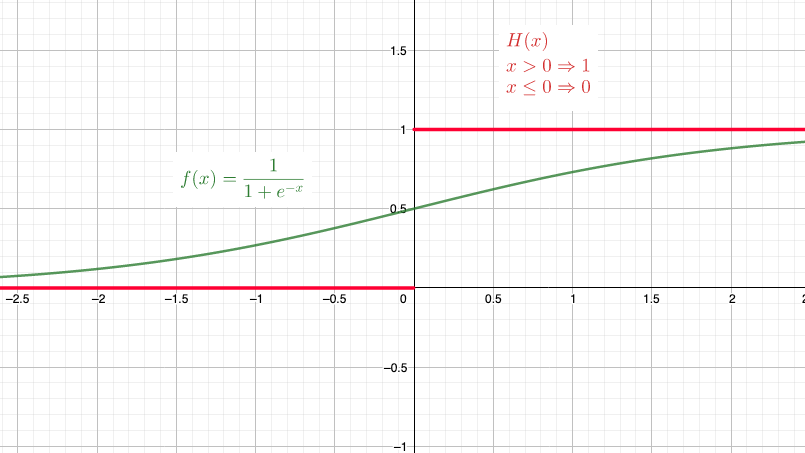
In order to geometrically explain how LSDMs disantangle, a possible approach is to make the (random) edge Bernoulli random variables, deterministic, by changing the link function. Indeed the sigmoid function is a smooth version of a non-continuous function, the Heaviside step function, given by $h(x) = \mathbb{1}_{{x>0}}$. This one yields an activation equal to 1 for positive inputs and 0 for negative inputs.

The deterministic graph is given by the following link indicators:
$\newcommand{\ind}{\mathbb{1}}$
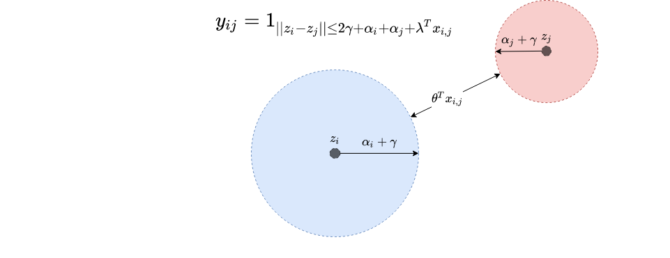
$$ y_{ij} = \ind_{ d(z_i,z_j) \leq 2\gamma +\alpha_i + \alpha_j+ \lambda^Tx_{ij}} $$
This one has a natural visual interpretation, as shown in the following image.

As can be seen, each embedding $z_i$ is endowed with a disk $D_i$ of radius $\alpha_i+\gamma$ such that the minimum distance between $D_i$ and $D_j$ in order for the nodes to connect is $\lambda^T x_{ij}$. If a given node has a large disk, it will naturally form more connections, independent on the position of the disk center.
Moreover the prior similarity between nodes $i$ and $j$ is high, then the disk need not be too close for the connection to form. As a consequence, the embeddings will not encode the prior information contained in the term $\lambda^T x_{ij}$.
Conclusion
In this article we focus on latent space distance models, and provide a visual interpretation of the mechanism that allow these models to learn vector representation of nodes that do not encode information known in advance in the form of node and edge attributes.
References
- Lovász, L. M. (2012). Large Networks and Graph Limits. Colloquium Publications.
- Hoff, P. D., Raftery, A. E., & Handcock, M. S. (2002). Latent space approaches to social network analysis. Journal of the American Statistical Association, 97(460), 1090–1098. https://doi.org/10.1198/016214502388618906